Linear Regression

Consider a bunch of error prone measurements $y_i$ made under different conditions conditions $\bold{x_i}$ that should have been related linearly as $y_i = \theta_1 f_1(x_{1i}) + \theta_2 f_2(x_{2i}) + \dots \theta_n f_n(x_{ni}) = \bold{\boldsymbol\theta^Tf(x_i)}$ , but are instead related as $y_i = \boldsymbol\theta\bold{^Tf(x_i)}+\epsilon_i$. Usually, to minimise this error, you would make the measurement multiple times in the same conditions and then use the average of those measurements as your $y_i$ . In such a condition, due to the central limit theorem, $\epsilon_i$ would follow a Gaussian distribution $N(0,\sigma^2)$ if you had taken infinite number of such measurement under the same conditions . Notice we are assuming that the error, in limit, follows the same distribution for each $i$ ..basically $\epsilon _i$ are i.i.d. variables . Thus, the probability distribution for $y_i$ would be $N(\boldsymbol\theta^T\bold{f(x_i)},\sigma^2)$ . This is what should happen for the correct value of $\boldsymbol\theta$ .

The main problem is that we don’t know this correct $\boldsymbol\theta$ , and so what we do is that we pretend for any general value of $\boldsymbol\theta$ that it’s correct, in order to find the probability of our data being the way it is in that case, namely $p(\bold{y,X\;|\;\boldsymbol\theta}) = \prod _ip(y_i,\bold{x_i}\;|\;\boldsymbol\theta)$ , and then using this probability and Bayes’ rule, we find $p(\bold{\boldsymbol\theta\;|\;y,X})$, which is the probability that our guess for $\boldsymbol\theta$ is correct. Thus, although we don’t know the correct value of $\boldsymbol\theta$ , we can find the most probable value, and just go along with it, since it explains the data the best. Note that $p(y_i,\bold{x_i}\;|\;\boldsymbol\theta)$ is the probability of the event that we observed $y_i$ AND the conditions are $\bold{x_i}$ , given that $\boldsymbol\theta$ is its true value. This can be written as $p(y_i\;|\;\bold{x_i},\boldsymbol\theta)p(\bold{x_i|\boldsymbol\theta})$ . It’s safe to say that the conditions we have for the observation $\bold{x_i}$ and the way that the observations $y_i$ are related to these conditions, which is represented by $\boldsymbol\theta$ should be independent. Thus we can write $p(\bold{x_i|\boldsymbol\theta})=p(\bold{x_i})$ . And thus $p(\bold{y,X\;|\;\boldsymbol\theta}) = \prod _ip(y_i,\bold{x_i}\;|\;\boldsymbol\theta) = \prod _ip(y_i\;|\;\bold{x_i},\boldsymbol\theta)\prod_ip(\bold{x_i})$ . And so, after using Bayes’ rule, we would have

as all other terms are independent of $\boldsymbol\theta$ . So to find the most probable $\boldsymbol\theta$ , we just have to maximise $p(\boldsymbol\theta)\prod _ip(y_i\;|\;\bold{x_i},\boldsymbol\theta)$ .

Maximum Likelihood Estimate

A common way to simplify this expression is to set the prior distribution $p(\boldsymbol\theta)=1$ . The expression thus obtained is $L(\boldsymbol\theta) = \prod _ip(y_i\;|\;\bold{x_i},\boldsymbol\theta)$, which is the Likelihood for $\boldsymbol\theta$. Equivalently, we can minimise the negative log likelihood, which is given by

.Discarding a bunch of constants, we just have to minimise :

where $\bold{F}$ is the matrix made of the row vectors $\bold{f(x_i)}$ .

This is the loss function, divided by the number of observations is known as the Means Squared Error.

Differentiating this loss function wrt $\boldsymbol\theta$ , we get the gradient

This can be used for gradient descent directly. But in this case, we can find the solution directly by setting the gradient to 0

Maximum A Posteriori Estimation

Remember how we discarded $p(\boldsymbol\theta)$ by setting it to 1 ? We did so because we knew nothing about $\boldsymbol\theta$ . If we did know something, then we can get a better estimate. For example, if $\boldsymbol\theta$ has a Gaussian distribution $N(\bold{0},b^2\bold{I})$ , then we get a more general estimate :

Setting $b^2$ to $\infty$ , we get the previous estimate.

Linear regression in action

Importing libraries

from matplotlib.pyplot import *
from numpy import *

Example 1

Generating Data

x1 = 10+2*random.random((1000,1))
x2 = 1+3*random.random((1000,1))
sig = 0.3
noise = random.randn(1000)*sig
y = sin(2*pi*x1[:,0])+cos(2*pi*x2[:,0])+noise
X = concatenate((x1,x2),axis=1)
del x1,x2
X,X_test = X[:800,:] , X[800:,:]
y,y_test = y[:800] , y[800:]

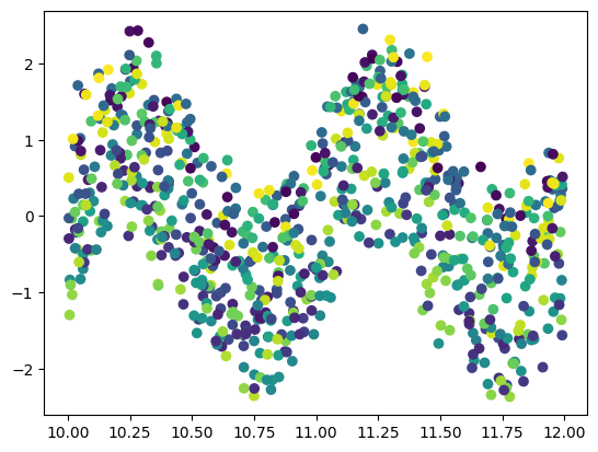
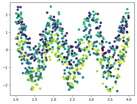
Plotting to get a feel

scatter(X[:,0],y,c=X[:,1])
figure()
scatter(X[:,1],y,c=X[:,0])

Now that we have figured out that the relationship is sinusoidal, we can assume $y = a\sin(x_1)+b\sin(x_2) + c\cos(x_1)+d\cos(x_2)$ and find the best value of $\boldsymbol{\theta} = [a\,b\,c\,d]^T$ .

def f(X):
    X = 2*pi*X
    return concatenate((sin(X[:,newaxis,0]),sin(X[:,newaxis,1]),cos(X[:,newaxis,0]),cos(X[:,newaxis,1])),axis=1)
F = f(X)
theta = dot(linalg.inv(F.T @ F) @ F.T ,y)
print(theta)

[ 1.02137996 -0.00515224 -0.05019073  1.02662538]

Predicting the values

def predict(X):
    global theta
    F = f(X)
    return dot(F,theta)
print("The error is :")
y_pred = predict(X_test)
print(mean((y_pred-y_test)**2))

The error is :
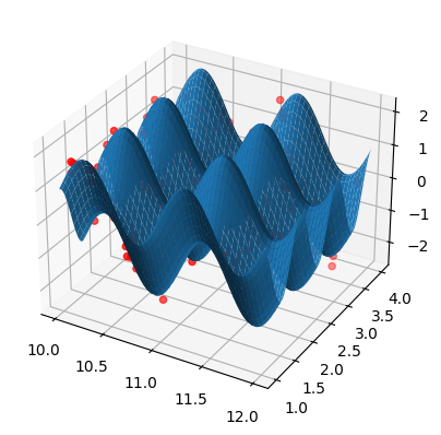
0.09683797274423349

A 3D plot showing the full picture

%matplotlib
fig = figure()
ax = fig.add_subplot(projection='3d')
X1 = tile(array([linspace(10,12,100)]),(100,1)) 
X2 = tile(array([linspace(1,4,100)]),(100,1)).T
Y = array([[predict(array([[X1[i,j],X2[i,j]]]))[0] for j in range(100)] for i in range(100)])
ax.plot_surface(X1,X2,Y,alpha=1)
ax.scatter3D(X_test[:,0],X_test[:,1],y_test,c='red')

Example 2

Generating Data

x = (2*random.random(100) - 1)*pi
x = x[:,newaxis]
X = ones((100,1))
for n in range(1,4):
    X = concatenate((X,x**n),axis=1)
y = sin(x)

We’ll consider the values of $x,x^2,x^3\dots$ to be the features (conditions of measurement) and $y$ to be observations.

theta = dot(linalg.inv(X.T @ X) @ X.T ,y)[:,0]
print(theta)
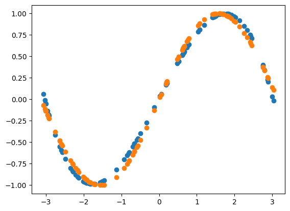
y_pred = [dot(theta,X[i]) for i in range(shape(X)[0])]
plot(x[:,0],y_pred,'o')
plot(x[:,0],y[:,0],'o')

[ 0.01508739  0.85071025 -0.00283029 -0.09259996]